In 1991, the USDA Forest Service, Southeastern Forest Experiment Station created a set of stem-profile taper models for 58 southern species and species groups. The Research Paper, known as SE-282, can be downloaded here. The research demonstrates how profile models are used to “predict stem diameter at any height” and “solve for volume to a given height or diameter”.

The limitations of the presented model are the vast number of parameters involved for each species/region combination, plus the complexity of the calculations required for each section of the stem (i.e.; butt, lower, middle and upper). To be useful in today’s business environment, the model needs to be incorporated into a software program.

So that’s where we’ll begin. In this post, I will explain how I selected a solution for implementing the model, and I will provide a simple use case for “how” and “why” someone might want to use this.

Converting the Model to a Python Package

Thinking about how I wanted to develop the model, I considered two alternatives, a Microsoft Excel workbook, and a Python package.

The drawbacks of the Excel approach were; multiple worksheets are needed to store all the parameters, numerous lookup functions result in deeply nested and confusing formulas, and the inability to automate the calculations over a large dataset of inputs. Technically this last one could be done using a VBA macro solution, but I’m not sure the additional complexity would be justified.

Considering the drawbacks with Excel, I decided to move forward with developing the model using the Python package format. Python packages can be easily shared with other users through Github, imported into various computing environments, including desktop, web and mobile solutions, as well as integrated with existing GIS software packages such as ArcGIS Pro and QGIS. The Python package I created is called STEMS.

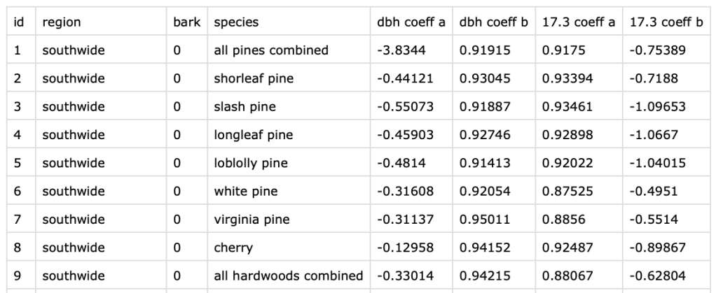
To incorporate the parameters into the model, I chose to store them in a SQLite database. SQLite databases have the advantage of being compact and self-contained (meaning easy to share and no installation required). The SQLite database was set up with a subset of the species/region parameters, but parameters for all 58 species and 8 regions can be easily added. Currently the database takes up about 25KB of storage, which is barely mentionable. A subset of the regression coefficients included in the Database, which are used to estimate diameter at DBH and 17.3 feet are included below.

Using the Model in Practice

A simple use case will help explain how to setup and use the model. But first, I’ll explain why someone might be interested in using it.

As indicated above, the intent is that the model will be used for estimating diameter at any height and volume (expressed in cubic feet) to given height or diameter. For the STEMS model, I converted the volume output from cubic feet to green tons using the weights per cubic foot presented in “Weights of Various Woods Grown in the United States“, USFS Technical Note 218, Madison, WI. This cannot be changed without modifying the underlying code, which anyone is free to do under the MIT license.

My expectation is that someone might want to use this to estimate cruise volumes, or analyze log merchandizing specifications in natural pine and hardwood stands. For instance, if a final harvest included multiple log specifications, you could analyze these to see how much volume and/or value it is expected to yield. This is the use case I will demonstrate here below.

Sample Scenario Setup:

The example scenario includes a tree length logging operation that will process Shortleaf pine logs to a 12″ top diameter inside bark, or a 14″ top diameter inside bark. The additional wood beyond these top sizes (i.e.; topwood) will be processed as rough top material to a 6″ top, with a little higher value than straight pulpwood. The landowner has been given the following prices: $46.50 per ton for the 12″ top log, $52.50 for the 14″ top log, and $10.00 for the top-wood.

The critical question will be, “If given the option to haul a 12″ or 14″ top diameter log, which should the landowner choose?” The stem-profile model only works on a single stem at a time. We could iterate over the model using a list or dataset of tree characteristics such as DBH and TOTAL HEIGHT, but for simplicity sake, let’s select an average tree to represent this harvest. Our example tree will be a Shortleaf Pine that is 20 inches DBH and 95 feet tall. The default for the model is to use inside-bark diameters, which is what we want. Let’s see how STEMS can be used to evaluate this decision.

'''Setup the model and retrieve the parameters from the database'''

# import stems
import stems

# create the Database Session
session = Session()

# create the model
spm = stems.StemProfileModel(spp='shortleaf pine', dbh=20, height=95)

# initialize the model parameters
spm.init_params(session)

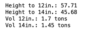
Now that the model is initialized and the parameters are stored, we can proceed to estimate our heights and volumes (tons) to 12″ and 14″ respectively.

# estimate height in feet to a 12" top log and a 14" top log
ht_to_12in = spm.estimate_stemHeight(d=12)
ht_to_14in = spm.estimate_stemHeight(d=14)

# estimate volume for each height
vol_12in = spm.estimate_volume(1, ht_to_12in)
vol_14in = spm.estimate_volume(1, ht_to_14in)

Output of the previous code.

Now we need to estimate the value for each stem, merchandized to a 12″ and 14″ top diameter, with a rough top log to a 6″ diameter.

# Estimate volume to a 6" top for topwood calcs.
ht_to_6in = spm.estimate_stemHeight(d=6)
vol_6in = spm.estimate_volume(1, ht_to_6in)

price_12in = 46.50
price_14in = 52.50
price_top = 10.0

rough_top_12 = spm.estimate_volume(ht_to_12in, ht_to_6in)
rough_top_14 = spm.estimate_volume(ht_to_14in, ht_to_6in)

value_12 = (vol_12in * price_12in) + (rough_top_12 * price_top)
value_14 = (vol_14in * price_14in) + (rough_top_14 * price_top)

Output of the previous code:

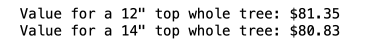
It’s as simple as that. We see that the most valuable product, assuming our average tree holds, is the 12″ top diameter scenario. If we expected 70 stems per acre looked similar to this, then we would be better off by $36.40 per acre, which could pay for the landowner’s herbaceous weed control application the following year. Now, we could make some additional assumptions, or “what if’s”, if we assumed that most of the stems were better or worse than average. Or the results might be skewed somewhat if there were a lot of sweep or defect in the logs. We could also estimate the proportion of top-wood volume to log volume. This would provide a basis for analyzing expected cutouts.

In my experience, under a tree length logging system, I’ve found that in most cases the landowner is more profitable when cutting to the largest top diameter allowed for a particular category of log (i.e.; chip-n-saw, plylog, and sawlog). Note also, that if we changed the 14″ diameter log price from $52.50 to $53.00, then the model predicts 14″ diameter logs are more profitable by about $0.20 per stem, or $14.00 per acre assuming 70 trees per acre as above. Obviously, we could do further sensitivity analysis to see what prices make these two merchandizing schemes equivalent.

As shown, having a reliable stem-profile model can be useful for providing analysis of stem merchandizing standards and prices. In addition to a flexible Python package that can be used in various environments, we also have the benefit of validation and error handling to ensure that the model is working correctly.

If you would like more information about STEMS, or to download the STEMS package for your own use, please visit my Github repository here.

Categories: Data Analytics Forest Inventory Forestry Apps Python

JwL