Foresters occasionally use inexpensive consumer grade GPS units for simple mapping tasks and navigation in the field. Many of these, such as the Garmin GPS Map series, retail for less than $300. I have owned several of these Garmin units myself , and have found them to be an invaluable tool for data collection.

Background Info:

Recently, I’ve been doing survival counts in our 2019 plantations. Survival counts are a common forest sampling activity that rely on tree count data from plots distributed within a plantation. These are typically done in the first year after planting. Foresters use this information to evaluate the current stocking (“trees per acre”) of recent plantations, to assess the condition of the planted trees (e.g.: stressed, healthy, etc), and to develop Silviculture plans.

I’ve done many of these survival counts in the past, but this time I wanted to document the location of each plot (e.g.; latitude and longitude). My reasoning was that the location data could be used to identify areas of high mortality within the plantation, and the data might correlate with conditions on the ground such as soil type limitations, slope, aspect, or drainage patterns.

The Process:

For this project, I used a Garmin GPS 64 unit to record the plot locations (i.e.; waypoints) in the field. Back at the office I downloaded the GPS unit using DNR GPS software, and exported the raw GPS data as an ESRI Shapefile. With the shapefile in hand, I was able to automate the inventory workup and visualizaion.

During the field inventory, I marked a waypoint at each plot center. I numbered the waypoint using a unique sequence which coincided with the plot number – 1 for the first plot, 2 for the second, etc. In the waypoint “Note” field I entered the tree count for the plot using the format planted/natural, where planted was the count of planted trees and natural was the count of natural trees on the plot. For example, for a plot with 8 planted trees and 3 natural trees, I entered 8/3 in the “Note” field for the waypoint.

I used Python code in a Jupyter Notebook environment for the data wrangling, inventory workup and analysis. The following Python packages were required; Pandas, GeoPandas, and NumPy for data processing, and Matplotlib and Folium for the mapping.

The GeoPandas package provides a geographically enabled Pandas DataFrame called a GeoDataFrame. The shapefile was imported into a GeoDataFrame using the following code.

# load the data and show the first five plots
FILENAME = '/field_plots/plots.shp'
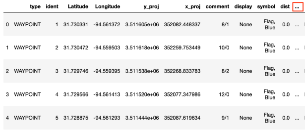
plots_full = gpd.read_file(FILENAME)

The next image shows the first five rows from the raw data read from the ESRI shapefile. The ellipsis (…) in the right corner indicates that this data contains more columns than displayed in the Jupyter Notebook.

Step 1: Filter out unnecessary columns.

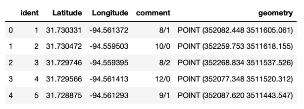
The resulting GeoDataFrame object had forty-four attributes (i.e.; columns), most of which were unnecessary for this analysis. Only five attribute columns were retained, these included:

• “ident” – identifies the waypoint. This is the value corresponding with the waypoint name.
• “Latitude” – the latitude value in decimal degrees format for each point.
• “Longitude” – the longitude value in decimal degrees format for each point.
• “comment” – contains the plot count data in the format planted/natural. DNR GPS renames the waypoint “Note” field to comment.
• “geometry” – this stores the spatial object, geometry type (Point). This column is required for a GeoDataFame object.

The next image shows the first five rows of the GeoDataFrame after selecting only these five columns.

Step 2: Separate the planted and natural counts in the comment field.

The text values in the “comment” field had to be separated into columns for the inventory workup phase. I used a Python function to parse these two values. This function is hardcoded to work with data separated using a “/”. In production code, this would likely be modified to allow users to indicate any valid character as a separator, provided that the plot data was recorded using that character.

def split_comment(row):
    '''split comment field and return a series with int values'''
    a, b = row.split("/")
    return pd.Series({'planted_cnt': int(a), 'natural_cnt': int(b)})

# add two new columns by applying the function above
plots[['planted_cnt', 'natural_cnt']] = plots.apply(lambda x: split_comment(x['comment']), axis=1)

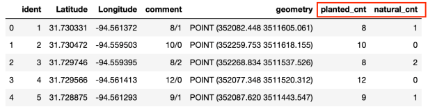
The next image shows the resulting GeoDataFrame. Notice the two additional columns “planted_cnt” and “natural_cnt”.

Step 3: Calculate the results.

The following code block shows the calculations on the GeoDataFrame to workup the inventory results.

# calculate means (mult by 50 for the expansion factor)
planted_mean = round(plots.planted_cnt.mean() * 50, 0)
natural_mean = round(plots.natural_cnt.mean() * 50, 0)

# calculated stats for planted trees
planted_std = round(plots.planted_cnt.std() * 50, 0)
planted_std_err = round(planted_std / plots.planted_cnt.count() ** 0.5, 2)
planted_ci_lower = round(planted_mean - 2 * planted_std_err, 0)
planted_ci_upper = round(planted_mean + 2 * planted_std_err, 0)
planted_coeff_var = round((planted_std / planted_mean) * 100, 2)
planted_sample_err = round((2 * planted_std_err / planted_mean) * 100, 2)

The next image shows the output of this step.

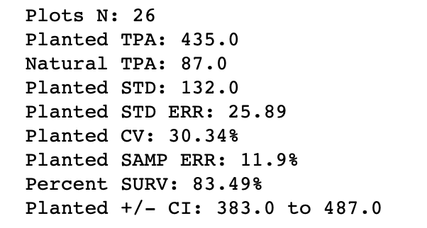
Notice the results show that the planted trees from our inventory averaged 435 per acre, compared to the 519 that were initially planted. Therefore, the survival was 83.5% of the initial planting density for this plantation. Overall this is not bad, but it could be better.

Also, the Sampling Error is above 10%, which is a common threshold for forest inventories. For survival counts, I doubt this is critical, but a few more plots in this plantation may have improved the results slightly.

The Confidence Interval (95%) surrounding the mean is +/- 52 trees per acre. This tells us that the average is likely to be within the range 383 to 487 trees per acre. We also had 87 trees per acre natural pine seed-in, which indicates that these natural seedlings should have been addressed in our site preparation prior to planting. These are just a few examples of the information we can derive from survival inventories.

Step 4: Visualize the Plots

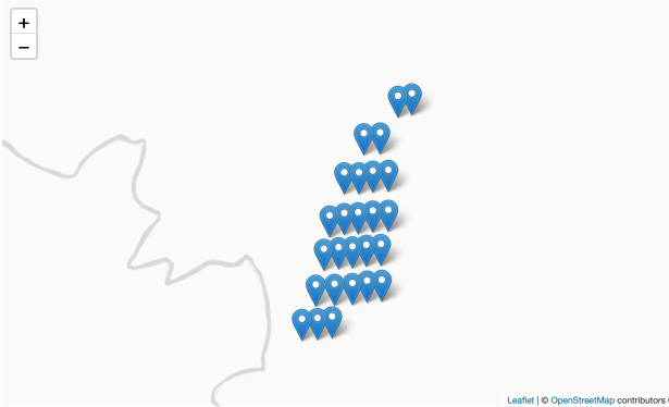
As indicated above, the Folium package was used to create maps to help visualize the plot locations. The following code was used to create a basic plot map using blue markers.

# find the midpoint of the data, use lat/lon for centering
mid_point = len(plots) // 2
center_of_map = [plots.iloc[mid_point]['Latitude'], plots.iloc[mid_point]['Longitude']]

# create a map showing plot locations
m_1 = folium.Map(location=center_of_map, tiles='cartodbpositron', zoom_start=14)

# add points to the map
for idx, row in plots.iterrows():
    Marker([row['Latitude'], row['Longitude']], popup=f"Plot: {row['ident']}").add_to(m_1)

embed_map(m_1, 'm_1.html')

Notice that the plots locations are on a systematic grid. This particular grid was 10 chains between lines and 4 chains between plots. Therefore, each plot represents a 4 acre sample.

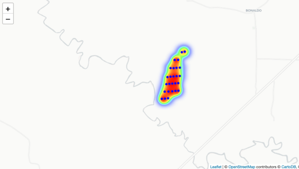
A heat map was created to visualize the intensity of tree count values across the landscape using the following code.

# Heat Map showing plot locations overlaid
m_2 = folium.Map(location=center_of_map, tiles='cartodbpositron', zoom_start=14)

# create a bubble map of the plots
for i in range(0, len(plots)):
    Circle(
        location=[plots.iloc[i]['Latitude'], plots.iloc[i]['Longitude']],
        radius=20,
        color='blue',
        popup=f'Tree Count: {plots.iloc[i]["planted_cnt"]}').add_to(m_2)
    
# create a heatmap
HeatMap(data=plots[['Latitude', 'Longitude', 'planted_cnt']], radius=18).add_to(m_2)

embed_map(m_2, 'm_2.html')

Here is the heat map at a small scale. Red areas have higher tree count values relative to the yellow and green areas.

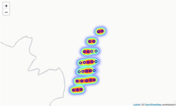
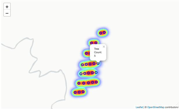
And one showing a larger scale. Notice we can also click on the plot (shown as a “o” on the map) and see the tree count for that plot.

Step 5: The final analysis

In this example, notice that there were only a few (three or four) plots in the green or yellow areas. Overall, the plot count was sufficient for this inventory, indicated by the amount of red areas relative to green areas.

But, looking closer at the heat map, the rightmost two plots on the third row from the top, and the rightmost plot on the fourth row from the top, were all located in a wet, low-lying area of the plantation. The soil in this area was saturated at the time of planting, and again when I completed the survival count. This area likely stays wet throughout the year, especially following big rain events. This could indicate that a small area of this plantation (7-10 acres) might have benefitted from bedding. We would likely need to look at the economics to determine if the expense of bedding would be justified to get better tree survival for this small area. Nevertheless, it is worth consideration.

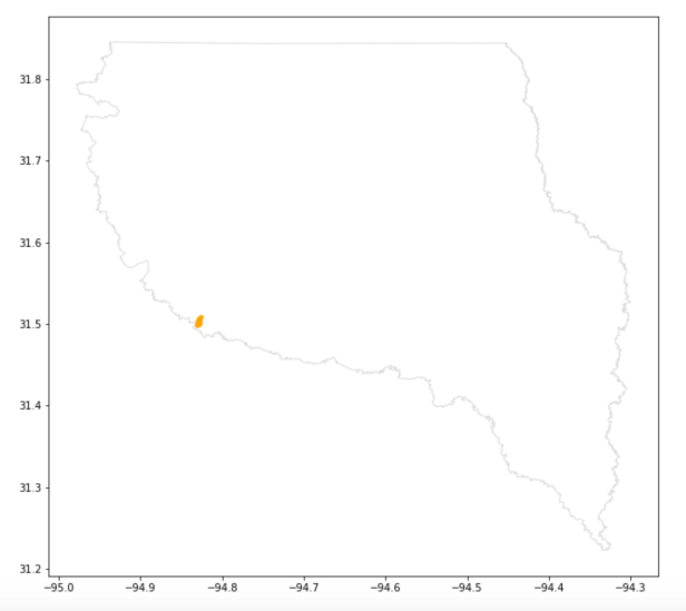
The final map shows the location of our inventory plots overlaid on a County map. Granted this isn’t the most practical map for a single inventory, but with more plot data it might be possible to correlate survival rates with drought patterns at the County, or sub-County, level.

Conclusion:

In this post we discussed how to collect survival inventory plots using a Garmin GPS unit. We wrangled the data using Python code in a Jupyter Notebook environment, calculated the inventory results, and created heat maps for further analysis of our tree counts.

This particular inventory showed good survival that was evenly distributed throughout the plantation, so there was little cause of concern regarding the previous Silviculture. Nevertheless, it’s interesting to note how much additional insight we gained from a simple survival count by adding the plot location component. Also, it was interesting that we could automate the inventory workup through Python code by encoding the plot tree count values into the Note field of the GPS waypoint.

Hopefully, this subject wasn’t too technical for the reader. In future posts, I’d like to include more subjects about automating workflows, data analytics and improving fieldwork processes within a Forestry setting. I believe foresters of the future will gradually become more dependent on technology, and will need to look for new ways to become more efficient on the job.

Categories: Data Analytics Forest Inventory

Tagged as: Data Analysis Forest Inventory Garmin GPS

JwL